

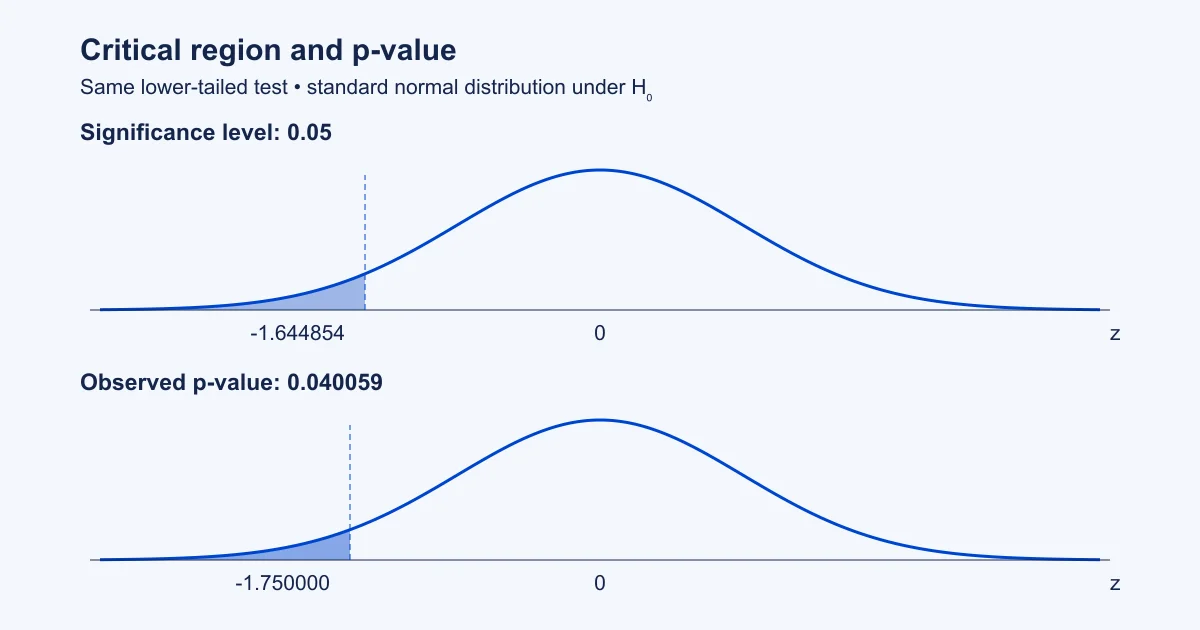
A p-value only becomes useful when you know which population claim you are testing and which tail answers the question.
This guide helps Singapore JC students connect their H2 Math calculator output to hypotheses, a rejection decision and a conclusion in context.
Work through one original example using both p-values and critical regions, then see why a different alternative can change the decision even with the same sample.
Define the population mean and choose the alternative before using the sample result.
Check the sampling assumptions and distinguish population standard deviation from standard error.
A p-value and a critical region give the same decision when the model, tail and significance level agree.
A non-rejection means insufficient evidence for the alternative; it does not prove the null hypothesis.
Start with the population mean, not the calculator
A hypothesis test asks whether sample evidence is sufficiently inconsistent with a specified population claim. The hypotheses concern an unknown population parameter. The sample supplies evidence; it is not the parameter being tested.
Let $\mu$ be the population mean and let $\mu_0$ be the value claimed under the null hypothesis. Write $H_0:\mu=\mu_0$. The alternative describes the question you are investigating:
- A decrease: $H_1:\mu<\mu_0$, so use the lower tail.
- An increase: $H_1:\mu>\mu_0$, so use the upper tail.
- A change in either direction: $H_1:\mu\ne\mu_0$, so use two tails.
Choose this direction from the question before inspecting the sample result. A sample mean below the claimed value does not turn a question about “a change” into a lower-tailed test. Define what the population mean measures, including its units, before writing the hypotheses.
Check which H2 test the question supports
This guide follows the 2026 SEAB H2 Mathematics syllabus, section 6.5, page 13. It covers tests of a population mean using a normal population with known variance, or a large sample from a population. The main example below uses the first case.
For independent observations from a normal population with mean $\mu$ and known variance $\sigma^2$, the sample mean has distribution
$$\bar X\sim\mathrm{N}\left(\mu,\frac{\sigma^2}{n}\right).$$
The second parameter in this notation is the variance. The standard deviation of the sample mean, also called its standard error, is $\sigma/\sqrt n$. Under $H_0$,
$$Z=\frac{\bar X-\mu_0}{\sigma/\sqrt n}\sim\mathrm{N}(0,1).$$
For a sufficiently large random sample, a normal approximation for the sample mean can be justified by the Central Limit Theorem under the usual independence and finite-variance conditions. If the population variance is unknown, use its unbiased estimate from the sample when applying the large-sample method. For observations $x_1,\ldots,x_n$, this is
$$s^2=\frac{\sum_{i=1}^{n}(x_i-\bar x)^2}{n-1}.$$
Do not forget the unbiased variance correction. The phrase “sample variance” is used with different conventions, so check its divisor. If the variance supplied or calculated from the sample uses divisor $n$, denote it here by $v_n$:
$$v_n=\frac{1}{n}\sum_{i=1}^{n}(x_i-\bar x)^2.$$
The unbiased estimate of the population variance is then
$$s^2=\frac{n}{n-1}v_n.$$
For example, if $n=40$ and the variance calculated with divisor $n$ is ${7.8\text{ cm}^2}$, the unbiased estimate is
$$s^2=\frac{40}{39}(7.8)=8\text{ cm}^2.$$
Using 7.8 directly misses the correction. The estimated standard error of the mean is $\sqrt{8/40}\approx0.4472$ cm, not $\sqrt{7.8/40}\approx0.4416$ cm. The smaller, uncorrected value makes the magnitude of the test statistic too large when the observed mean differs from the null mean, and can affect a borderline decision.
If a calculator gives a sample standard deviation $s_x$ calculated using divisor $n-1$, its square already gives the unbiased variance estimate. Do not multiply that square by $n/(n-1)$ again. If the given quantity is a standard deviation calculated using divisor $n$, square it first, then apply the correction. An estimate is still an estimate; it does not become the known population variance.
The corresponding standard error is estimated by $s/\sqrt n$, and the normal test is approximate. Do not silently replace a known population standard deviation with a sample estimate. A small sample with unknown population variance is not the case taught here. The sampling background is in section 6.4, page 12.
Original example: is a filling machine underfilling?
A machine is intended to fill bottles with a population mean volume of 500 ml. The volume filled is modelled by a normal distribution with known standard deviation 8 ml. A random sample of 25 bottles is selected, and the observations may be treated as independent. The sample mean is 497.2 ml. Test, at the 5% significance level, whether the population mean volume is below 500 ml.
This is an invented teaching example, not a report about a real manufacturer.
Let $\mu$ be the population mean volume, in ml, filled by the machine under these operating conditions. Then
$$H_0:\mu=500,\qquad H_1:\mu<500.$$
Use a lower-tailed test with significance level $\alpha=0.05$. Normality is given, the population variance is known, and independence is assumed. The sample size of 25 does not require a large-sample approximation here: a mean of independent normal observations is itself normal.
Under $H_0$,
$$\bar X\sim\mathrm{N}\left(500,\frac{8^2}{25}\right)=\mathrm{N}(500,2.56).$$
The standard error is ${8/\sqrt{25}=1.6}$ ml. The observed standardised test statistic is
$$z=\frac{497.2-500}{1.6}=-1.75.$$
This says the observed sample mean is 1.75 standard errors below the null mean. It does not yet say whether that is sufficient evidence at the chosen significance level.
Method 1: calculate and interpret the p-value
The p-value is the probability, assuming the null hypothesis and the test model, of a test statistic at least as extreme as the observed one in the direction or directions specified by the alternative. See NIST’s explanation of p-values and critical values.
For this lower-tailed test,
$$p=\mathrm{P}(Z\le-1.75)=0.040059\ldots\approx0.0401.$$
Equivalently, calculate $\mathrm{P}(\bar X\le497.2)$ under $\bar X\sim\mathrm{N}(500,2.56)$.
Since ${0.040059\ldots<0.05}$, reject $H_0$. At the 5% significance level, there is sufficient evidence that the population mean volume filled by the machine is below 500 ml.
Under the null model, about 4.01% of samples of this size would give a mean no greater than 497.2 ml. This is not a 4.01% probability that the null hypothesis is true. It is not the percentage of bottles below 500 ml, and it does not prove that every bottle is underfilled.
Method 2: find the critical region
A critical region is the set of test-statistic values for which the decision rule rejects the null hypothesis. Set the boundary using the significance level, rather than the observed result.
For a lower-tailed 5% test, find $c$ such that
$$\mathrm{P}(Z\le c)=0.05.$$
The critical value is $c=-1.6448536\ldots$. Thus the rejection rule is
$$Z\le-1.6448536\ldots.$$
The observed value $-1.75$ lies in that region, so reject $H_0$, giving the same contextual conclusion as the p-value method.
You can express the same boundary in the original units. Under the null model, the lower 5% cutoff for sample means is
$$\begin{aligned}500+1.6(-1.6448536\ldots)\\{}=497.368234\ldots\text{ ml}.\end{aligned}$$
So the critical region is $\bar X\le497.368234\ldots$ ml. The observed mean, 497.2 ml, lies inside it. This is a cutoff for a sample mean of 25 bottles, not an individual bottle.
The significance level describes the long-run probability of rejecting the null hypothesis when the null model is true. In this exact continuous test the critical region has probability 0.05 under that model. The p-value instead uses the observed result as its tail boundary: its area is approximately 0.0401. The diagram compares those two areas.
Keep extra digits in the calculator and round only for presentation. A displayed p-value of 0.050 may have come from either side of 0.05; inspect more digits before deciding. This guide uses the rule “reject when $p\le\alpha$”. For this continuous model, including the exact cutoff does not change the tail probability because a single value has probability zero.
Calculator inputs: keep the distribution and units consistent
Use the normal cumulative probability and inverse-normal functions on your calculator. These instructions describe the mathematical inputs; menu names and argument order vary by model.
- Standardised p-value: choose a normal distribution with mean 0 and standard deviation 1; calculate its lower-tail probability up to −1.75. The output should be approximately 0.040059.
- Unstandardised cross-check: choose mean 500 and standard deviation 1.6; calculate its lower-tail probability up to 497.2. The output should be the same.
- Critical value: choose an inverse-normal calculation with left cumulative area 0.05, mean 0 and standard deviation 1. The result should be approximately −1.644854.
- Cutoff in ml: choose left cumulative area 0.05, mean 500 and standard deviation 1.6. The result should be approximately 497.368234.
For a cumulative function requiring both bounds, use the calculator’s documented way of representing a lower bound of negative infinity. Check whether the screen asks for a left-tail area, right-tail area, or interval. An inverse-normal left area of 0.95 gives a positive critical value, which is not the lower-tail boundary needed here.
If using a built-in one-sample Z-test in summary-statistics mode for this example, the inputs are null mean 500, population standard deviation 8, sample mean 497.2, sample size 25 and alternative “less than”. That routine forms the standard error itself. Do not enter 1.6 as its population standard deviation: 1.6 belongs in the direct sample-mean distribution calculation above.
Write the hypotheses, distribution, probability statement or rejection boundary, comparison and contextual conclusion in your working. A calculator screen does not explain why you selected that tail. Follow any question-specific working instructions; SEAB’s calculator guidance is on page 4.
Same data, different question: a two-tailed test
Now suppose the question had instead been set in advance as: “Has the population mean volume changed from 500 ml?” Keep the model and sample data the same, but use
$$H_0:\mu=500,\qquad H_1:\mu\ne500.$$
Both unusually low and unusually high sample means count against the null hypothesis. The observed statistic is still $z=-1.75$. By symmetry of the standard normal distribution,
$$p=2\mathrm{P}(Z\le-1.75)=0.080118\ldots.$$
Since $p>0.05$, do not reject $H_0$. At the 5% significance level, there is insufficient evidence that the population mean volume differs from 500 ml. This does not establish that the mean equals 500 ml.
The equivalent two-tailed critical region places 0.025 in each tail:
$$Z\le-1.959964\ldots\quad\text{or}\quad Z\ge1.959964\ldots.$$
The observed $-1.75$ is outside that region. A one-tailed rejection and a two-tailed non-rejection are consistent here because the tests ask different questions and use different rejection boundaries. You must not switch to the one-tailed question after seeing which gives a rejection.
For an upper-tailed question such as whether a new setting increases the mean above 500 ml, use $H_1:\mu>500$. If the observed statistic were $+1.75$, the p-value would be $\mathrm{P}(Z\ge1.75)\approx0.0401$. With the original negative statistic, however, the upper-tail p-value would be $\mathrm{P}(Z\ge-1.75)\approx0.9599$: the data point in the opposite direction.
An error checklist before you finish
- Testing the sample mean: replace a hypothesis about $\bar x$ with one about the defined population mean $\mu$. The sample mean is already observed.
- Using the wrong spread: normal notation uses variance, whereas many calculator input screens ask for standard deviation. Here these are 2.56 and 1.6 for the sample mean.
- Missing the unbiased variance correction: if the sample variance uses divisor $n$, multiply it by $n/(n-1)$ before using it to estimate the population variance. If it already uses divisor $n-1$, do not correct it again.
- Dividing twice: a Z-test routine needs the population standard deviation; a direct normal calculation for the sample mean needs the standard error.
- Choosing the tail from the answer: read the alternative before looking at the sign of the statistic.
- Doubling every probability: doubling the matching one-tail area is appropriate for the symmetric two-sided normal test here, not for a one-tailed test.
- Claiming normality because a sample is large: the approximation concerns the distribution of the sample mean, not the distribution of individual observations.
- Writing “accept the null”: write “do not reject” and explain that evidence for the alternative is insufficient at the stated level.
- Confusing significance with size: the estimated shortfall is 2.8 ml. Whether that matters operationally is a separate question from the statistical decision.
- Ignoring the sampling assumptions: repeated measurements from the same bottle or a convenience sample require scrutiny; a probability calculation does not repair a poor sampling design.
To diagnose your own work, cover the numerical solution and write just the parameter, hypotheses, assumptions and tail. Then calculate. Finally, write a conclusion that names the population mean, direction and significance level.
Try one question without copying the conclusion
A machine produces rods whose lengths are normally distributed with known standard deviation 0.6 cm. An independent random sample of 36 rods has mean length 20.18 cm. At the 5% significance level, test whether the population mean length is greater than 20 cm.
Worked answer. Let $\mu$ be the population mean rod length in cm. Use $H_0:\mu=20$ and $H_1:\mu>20$. Under $H_0$, $\bar X\sim\mathrm{N}(20,0.01)$ and
$$z=\frac{20.18-20}{0.6/\sqrt{36}}=1.8.$$
The upper-tail p-value is $\mathrm{P}(Z\ge1.8)=0.035930\ldots<0.05$, so reject $H_0$. There is sufficient evidence at the 5% significance level that the population mean rod length is greater than 20 cm.
As a cross-check, the upper-tail critical value is ${1.6448536\ldots}$. In cm, the rejection boundary is ${20+0.1(1.6448536\ldots)=20.164485\ldots}$. The observed mean exceeds that boundary.
Connect this method to your H2 revision
If you could calculate the probability but not justify the tail, practise writing the setup for several questions before doing any arithmetic. If the spread was wrong, revisit the distribution of the sample mean before repeating whole tests.
Use the H2 Math revision-order guide to fit that repair into your wider study plan. Keep the MF27 formula booklet available when reviewing normal-distribution notation, but choose the hypotheses and interpret the conclusion yourself: a formula reference cannot make those decisions for you.
If you need feedback on why your setup or conclusion is incomplete, explore H2 Math lessons at Tim Gan Math. Bring an attempted solution so the discussion can focus on the exact step that needs attention.
Conclusion
A complete hypothesis test connects a population question to a model, a tail probability or boundary, and a qualified conclusion.
Action Steps:
Write the setup before opening the calculator menu.
Check one p-value using both standardised and original units.
Rewrite your conclusion so that it names the population mean and the significance level.
Practise explaining why each line is there. That makes the method reusable when the context changes.